40 add data labels to pivot chart

How to Use Excel Pivot Table Label Filters Watch the steps in this short video, and the written instructions are below the video. Play. To change the Pivot Table option to allow multiple filters: Right-click a cell in the pivot table, and click PivotTable Options. Click the Totals & Filters tab Under Filters, add a check mark to 'Allow multiple filters per field.'. Adding Data Labels to a Pivot Chart with VBA Macro ActiveSheet.ChartObjects ("Cluster Overview").Activate ActiveChart.FullSeriesCollection (1).DataLabels.Select For i = 1 To Range ("PivotTable1 [Project '#]").Count ActiveChart.FullSeriesCollection (1).Points (i).DataLabel.Select Selection.Formula = Range ("PivotTable1 [Project '#]").Cells (i, 1) Next i Any help you can give will be great.

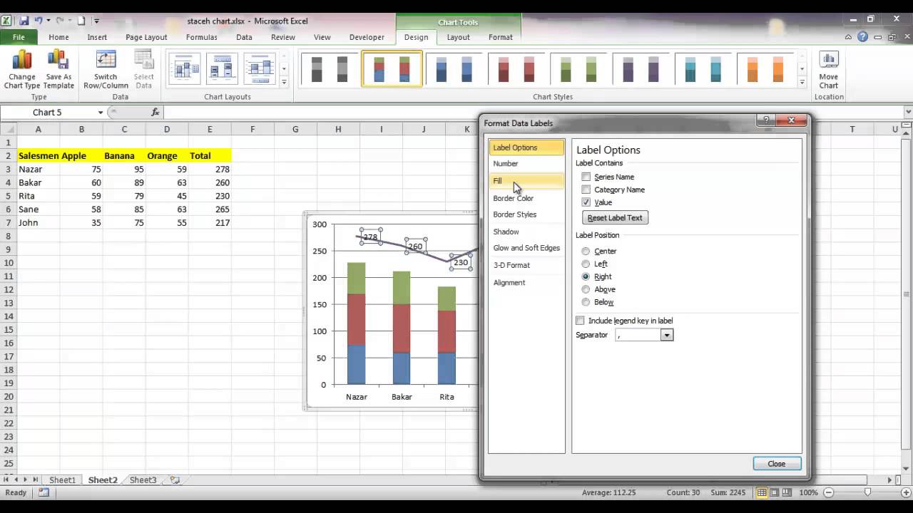
How to Customize Your Excel Pivot Chart Data Labels - dummies To add data labels, just select the command that corresponds to the location you want. To remove the labels, select the None command. If you want to specify what Excel should use for the data label, choose the More Data Labels Options command from the Data Labels menu. Excel displays the Format Data Labels pane.

Add data labels to pivot chart

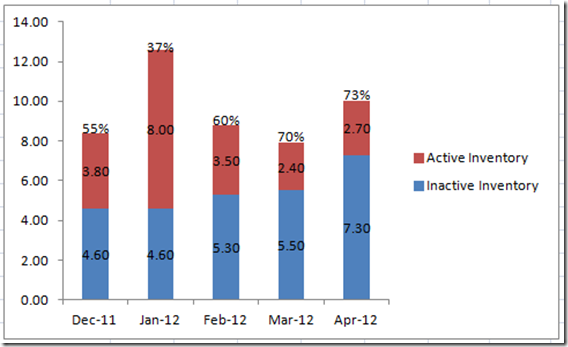
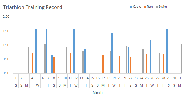
Automatic Row And Column Pivot Table Labels Select the data set you want to use for your table The first thing to do is put your cursor somewhere in your data list Select the Insert Tab Hit Pivot Table icon Next select Pivot Table option Select a table or range option Select to put your Table on a New Worksheet or on the current one, for this tutorial select the first option Click Ok Add a DATA LABEL to ONE POINT on a chart in Excel Steps shown in the video above: Click on the chart line to add the data point to. All the data points will be highlighted. Click again on the single point that you want to add a data label to. Right-click and select ' Add data label ' This is the key step! Right-click again on the data point itself (not the label) and select ' Format data label '. Include Grand Totals in Pivot Charts - My Online Training Hub Step 5: Format the Chart. The Grand Total value is the top segment of the stacked column chart. We need to hide this, but first let's select the grand total series and add Data Labels > Inside Base: Next, with the grand total series still selected go to the Format tab > Shape Fill > No Fill. Hide the gridlines and vertical axis, and place the ...

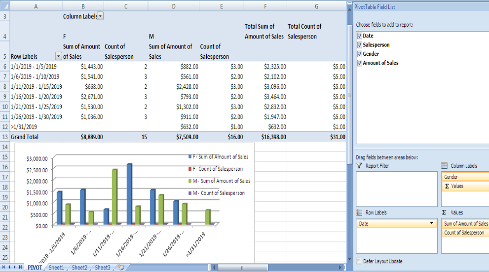
Add data labels to pivot chart. Adding rich data labels to charts in Excel 2013 - Microsoft 365 Blog Putting a data label into a shape can add another type of visual emphasis. To add a data label in a shape, select the data point of interest, then right-click it to pull up the context menu. Click Add Data Label, then click Add Data Callout . The result is that your data label will appear in a graphical callout. Add Percentage to Pivot Table | MyExcelOnline Here is how the Pivot Table Percentage looks like: STEP 3: Click the second Sales field's (Sum of SALES2) drop down and choose Value Field Settings. STEP 4: Select the Show Values As tab and from the drop down choose % of. For the Base Field pick Financial Year. For the Base Item pick (previous). This means we want to get the % of values ... How to Add Data to a Pivot Table: 11 Steps (with Pictures) You can do this in both Windows and Mac versions of Excel. Steps Download Article 1 Open your pivot table Excel document. Double-click the Excel document that contains your pivot table. It will open. 2 Go to the spreadsheet page that contains your data. Click the tab that contains your data (e.g., Sheet 2) at the bottom of the Excel window. 3 How to add Data Labels to my PivotChart form | PC Review Access Chart Data label: 1: Aug 30, 2005: Change name of labels in a PivotChart: 4: Jul 7, 2008: PivotChart print from form: 1: May 20, 2008: Data labels on PivotCharts shown as Integers, I need 2 Decimal Pla: 2: Mar 31, 2005: Sort numbers stored as texts as numbers: 3: Sep 18, 2007: How do I copy a pivotChart to paste into another doc? 1: Dec ...

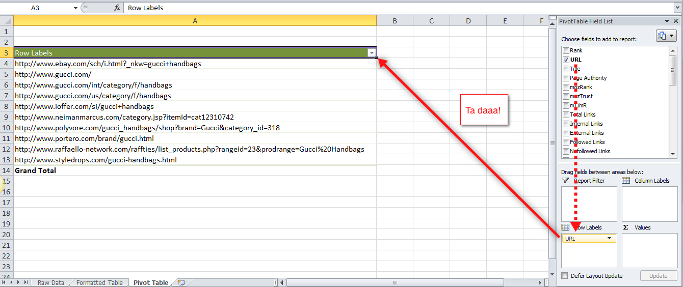
Pivot table - Wikipedia Table that summarizes data from another table. For cross-tabulation that aggregates only by counting (rather than summing, averaging, etc.), see Contingency table. A pivot table is a table of grouped values that aggregates the individual items of a more extensive table (such as from a database, spreadsheet, or business intelligence program ... Create Dynamic Chart Data Labels with Slicers - Excel Campus You basically need to select a label series, then press the Value from Cells button in the Format Data Labels menu. Then select the range that contains the metrics for that series. Click to Enlarge Repeat this step for each series in the chart. If you are using Excel 2010 or earlier the chart will look like the following when you open the file. Add a data label on Pivot Chart - social.technet.microsoft.com With .SeriesCollection (1).Points (i) .HasDataLabel = True .DataLabel.Text = Worksheets ("Sheet2").Range ("a" & position_total).Value position_total = position_total + 1 End With End With Next End Sub Select the Pivot chart, then run the macro "data_label". Jaynet Zhang TechNet Community Support How to make row labels on same line in pivot table? Make row labels on same line with PivotTable Options You can also go to the PivotTable Options dialog box to set an option to finish this operation. 1. Click any one cell in the pivot table, and right click to choose PivotTable Options, see screenshot: 2.

How to add Data label in Stacked column chart of Pivot charts I'm tring to make a Pivot chart with stacked column graph. In where, i couldn't add data label for cumulative sum of value in Data label. Where i could only add data label to individual stacks in column graph. It found possible with normal stacked column chart without pivot chart. How to update or add new data to an existing Pivot Table in Excel And here's the resulting Pivot Table: Change the Source Data for your Pivot Table. In order to change the source data for your Pivot Table, you can follow these steps: Add your new data to the existing data table. In our case, we'll simply paste the additional rows of data into the existing sales data table. Change the format of data labels in a chart To get there, after adding your data labels, select the data label to format, and then click Chart Elements > Data Labels > More Options. To go to the appropriate area, click one of the four icons ( Fill & Line, Effects, Size & Properties ( Layout & Properties in Outlook or Word), or Label Options) shown here. Add Value Label to Pivot Chart Displayed as Percentage If you use the hidden line method: How to Add Total Data Labels to the Excel Stacked Bar Chart and then use the code mentioned in post #2 to create boxes offset from the hidden line points, you should be able to place the additional labels where you want. You must log in or register to reply here.

How-to Put Percentage Labels on Top of a Stacked Column Chart - Excel Dashboard Templates

How to Add Data Labels in Excel - Excelchat | Excelchat After inserting a chart in Excel 2010 and earlier versions we need to do the followings to add data labels to the chart; Click inside the chart area to display the Chart Tools. Figure 2. Chart Tools. Click on Layout tab of the Chart Tools. In Labels group, click on Data Labels and select the position to add labels to the chart.

Display Missing Dates in Excel PivotTables • My Online Training Hub

Formal ALL data labels in a pivot chart at once Hi AaronSchmid ，. I go through the post, as per the article: Change the format of data labels in a chart, you may select only one data labels to format it. However, you may change the location of the data labels all at once, as you can see in screenshot below: I would suggest you vote for or leave your comments in the thread: Format Data ...

How to Add Fields to Your Pivot Table | Excelchat

Pivot Charts with Data Labels other than Values Click on data labels and use the right "arrow" to select that you want the information to appear above the bar. Then right click on the data label and select Format Data Labels, Under label options you have choices like Series name, Category name, etc. One spreadsheet to rule them all. One spreadsheet to find them.

How To Manage Big Data With Pivot Tables

How to add data labels from different column in an Excel chart? Right click the data series in the chart, and select Add Data Labels > Add Data Labels from the context menu to add data labels. 2. Click any data label to select all data labels, and then click the specified data label to select it only in the chart. 3.

Add Total Label On Stacked Bar Chart In Excel - YouTube

Adding Data Labels to a Chart Using VBA Loops - Wise Owl To do this, add the following line to your code: 'make sure data labels are turned on. FilmDataSeries.HasDataLabels = True. This simple bit of code uses the variable we set earlier to turn on the data labels for the chart. Without this line, when we try to set the text of the first data label our code would fall over.

microsoft excel - How to make chart showing year over year, where fiscal year starts July ...

How to add data labels to pivot chart? | Console App Forums - Syncfusion The CSV data goes into the Data sheet and the application then creates a pivot table and corresponding pivot chart from this data in the Charts sheet. The chart is created alright but i see no option to add data labels to it using XlsIO. The chart is created as follows: IChartShape pivotChart = chartsSheet.Charts.Add();

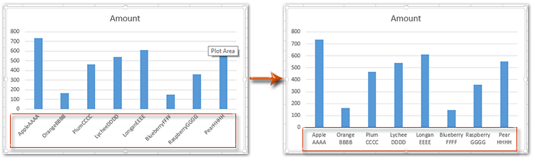
How to wrap X axis labels in a chart in Excel?

How to Add Data to a Pivot Table in Excel | Excelchat Setting up the Data We will create a Pivot Table with the Data in figure 2 Figure 2 - Setting up the Data Creating the Data Table Before creating the table, we will put the data into a table We will click on any part of the data We will click on the Insert tab and click on Table Figure 3- Clicking on Table Figure 4- Create Table Dialog box

Visualization of JIRA Issue Data in Confluence | Stiltsoft

How to Customize Your Excel Pivot Chart and Axis Titles The Chart Title and Axis Titles commands, which appear when you click the Design tab's Add Chart Elements command button in Excel, let you add a title to your chart titles to the vertical, horizontal, and depth axes of your chart. In Excel 2007 and Excel 2010, you use the Chart Title and Axis Titles commands on the Layout tab to add chart and axis titles. After you choose the Chart ...

Share :