38 conditional formatting pivot table row labels

How to Apply Conditional Formatting to Pivot Tables 13.12.2018 · Great question! I don’t believe there is a direct way to do this with the conditional formatting setting for the pivot table. Those settings are applied at the pivot field level, and not the pivot item level. In the example of Quarters, each quarter (Q1, Q2, Q3, Q4) would be a pivot item. The conditional formatting is applied at the field level. Conditional Formatting Using Custom Measure - Power BI 28.09.2020 · Let us consider the following table visual: I have got sales by clothing category, by day of a week in the above table visual. Now, my task is to give a custom conditional formatting to the Day of Week column above based on the Clothing Category. For example - Clothing Category = Jackets should be GREEN. Clothing Category = Jeans should be BLUE

How to Show Text in Pivot Table Values Area - Contextures Excel … 27.01.2022 · On the Excel Ribbon's Home tab, click Conditional Formatting; Then click New Rule, to open the New Formatting Rule dialog box; In the Apply Rule to section, select the 3rd option - All cells showing 'Max of RegID' values for 'City' and 'Store'. This option creates flexible conditional formatting that will adjust if the pivot table layout changes.

Conditional formatting pivot table row labels

Overwrite pivot table conditional format based on row label As far as I know, using the one rule in the Conditional formatting, we can only format the cells with one color if the condition is true and if the same condition is false, the formatting of the cell will be blank and if both conditions are true, the formatting of cell depends on the highest ranking/priority of the rules in Conditional formatting. Conditional Format Pivot Table Row - Chandoo.org Select the entire row, and when you apply the conditional format, make the column reference absolute. So, say we want the entire row 2 to be formatted if cell in col B = 5. formula would be: =$B2=5 101 Excel Pivot Tables Examples | MyExcelOnline 31.07.2020 · Pivot Tables in Excel are one of the most powerful features within Microsoft Excel. An Excel Pivot Table allows you to analyze more than 1 million rows of data with just a few mouse clicks, show the results in an easy to read table, “pivot”/change the report layout with the ease of dragging fields around, highlight key information to management and include Charts & …

Conditional formatting pivot table row labels. Conditional formatting rows in a pivot table based on one rows criteria ... I am havong difficulty trying to highlight an entire row in a pivot table based on one rows criteria. The pivot table is from A:M and I need to highlight the corresponding row if column I has 992 in it. I have tried sevral ways but can only get it to work if I just focus on one row. I am at a loss for what I am doing wrong. Pivot table conditional formatting based on row label Kerja, Pekerjaan ... Cari pekerjaan yang berkaitan dengan Pivot table conditional formatting based on row label atau upah di pasaran bebas terbesar di dunia dengan pekerjaan 21 m +. Ia percuma untuk mendaftar dan bida pada pekerjaan. Conditional Formatting PivotTables • My Online Training Hub Here's a step by step how to: 1. Select any cell in the values area of your PivotTable. 2. On the Home tab of the Ribbon select Conditional Formatting > Top/Bottom Rules > Top 10 Items: 3. Set the value to 1 and choose your format: 4. You will now have an icon beside the cell that you have applied the formatting to. › blog › insert-blank-rows-inHow to Insert a Blank Row in Excel Pivot Table | MyExcelOnline Jan 17, 2021 · STEP 1: Click any cell in the Pivot Table. STEP 2: Go to Design > Blank Rows. STEP 3: You will need to click on the Blank Rows button and select Insert Blank Line After Each Item. NB: For this to work you will need at least two Pivot Table Items in the Rows Labels. You then get the following Pivot Table report:

› blog › 101-excel-pivot-tables101 Excel Pivot Tables Examples | MyExcelOnline Jul 31, 2020 · Pivot Tables in Excel are one of the most powerful features within Microsoft Excel. An Excel Pivot Table allows you to analyze more than 1 million rows of data with just a few mouse clicks, show the results in an easy to read table, “pivot”/change the report layout with the ease of dragging fields around, highlight key information to management and include Charts & Slicers for your monthly ... Conditional Formatting on Pivot Table row labels Re: Conditional Formatting on Pivot Table row labels Hi Dilip, The date is a "date" and not a text. What I mean is each cell in A should be compared with the 3 dates in E and should do the conditional formatting (excel icon sets) accordingly. If you see the cell A in srcFromWorkSheet you know what I mean. Please let me know if you have any queries. Excel VBA: Conditional Format of Pivot Table based on Column Label ... myPivotSourceName = myPivotField.Name. Then rather than referencing the data field with the pivot field object, I referenced the DataRange with the string: myPivotTable.PivotFields (myPivotSourceName).DataRange.Select. Works perfectly and is completely portable for any pivottable on any sheet with any fields. excel vba. How to Insert a Blank Row in Excel Pivot Table | MyExcelOnline 17.01.2021 · Pivot Table reports are shown in a Compact Layout format as a default and if you have two or more Items in the Row Labels (e.g.Month & Customer), then the Pivot Table report can look very clunky…. There is a cool little trick that most Excel users do not know about that adds a blank row after each item, making the Pivot Table report look more appealing.

community.powerbi.com › t5 › Community-BlogConditional Formatting Using Custom Measure - Power BI Sep 28, 2020 · Let us consider the following table visual: I have got sales by clothing category, by day of a week in the above table visual. Now, my task is to give a custom conditional formatting to the Day of Week column above based on the Clothing Category. For example - Clothing Category = Jackets should be GREEN. Clothing Category = Jeans should be BLUE Pivot Table Conditional Formatting with VBA - Peltier Tech Here is PivotTable1 with the conditional formatting applied. Here is PivotTable2 with the same formatting applied. Note that refreshing the pivot tables changes values but does not automatically reformat the tables. You have to manually rerun the VBA routines, or capture the PivotTableUpdate event: Private Sub Worksheet_PivotTableUpdate (ByVal ... Pivot table conditional format based on row value Hi there, I am hoping there is a way to use conditional formatting to change the fill color of the data cells on a pivot table based on the row value. In the picture below you can see I have grouped some values together to form the row categories - I would like to tell excel to fill the cells... Apply conditional table formatting in Power BI - Power BI To format cell background or font color, select Conditional formatting for a field, and then select either Background color or Font color from the drop-down menu. The Background color or Font color dialog box opens, with the name of the field you're formatting in the title. After selecting conditional formatting options, select OK.

33 Pivot Table Blank Row Label - Labels Database 2020

How to Apply Conditional Formatting to Rows Based on Cell Value Start by deciding which column contains the data you want to be the basis of the conditional formatting. In my example, that would be the Month column (Column E). Select the cell in the first row for that column in the table. In my case, that would be E6. On the Home tab of the Ribbon, select the Conditional Formatting drop-down and click on ...

Conditional Formatting

Add Pivot Table Conditional Formatting and Fix Problems On the Ribbon's Home tab, click Conditional Formatting, then click Manage Rules In the list of rules, select the Data Bar rule, which applies to cells B3:B8 Click Edit Rule, to open the Edit Formatting Rule window. In the Edit the Rule Description section, add a check mark to Show Bar Only

How to use conditional formatting in decorating pivot tables | Basic Excel Tutorial

Issue with conditional formatting in pivot table | General Excel ... No, you either have totals on or off for all columns. You could use some conditional formatting to hide the totals by formatting the font in the same colour as the total cell. You'd need to use regular conditional formatting for this, i.e. not PivotTable conditional formatting. Apply it to the column, where the row label contains 'Total'.

vba - Conditional Formatting in Pivot Table in Excel based on text field - Stack Overflow

Conditional Formatting in Pivot Table - WallStreetMojo We must follow the steps to apply conditional formatting in the pivot table. First, we must select the data. Then, in the "Insert" Tab, click on "Pivot Tables." As a result, a dialog box appears. Next, we must insert the pivot table in a new worksheet by clicking "OK." Currently, a pivot table is blank. Next, we need to bring in the values.

34 Using The Current Worksheets Pivot Table Add The Task Name As A Column Label - Labels ...

Apply Conditional Formatting | Excel Pivot Table Tutorial Go to Home Tab → Styles → Conditional Formatting → New Rule. From rule to, select the third option. And, from "select a rule" type select "Format only top or bottom" ranked values. In edit rule description, enter 1 in the input box and from the drop-down menu select "each Column Group". Apply formatting you want. Click OK.

How to use Conditional Formatting in the Pivot table | Excelinexcel

Pivot Table: Pivot table conditional formatting | Exceljet Select any cell in the data you wish to format and then choose "New rule" from the conditional formatting menu on the Home tab of the ribbon. At the top of the window, you will see setting for which cells to apply conditional formatting to. For the example shown, we want: "All cells showing sum of "sales values" for name and "date"

How to Create a MS Excel Pivot Table – An Introduc

› pivot-tables › pivot-tableHow to Apply Conditional Formatting to Pivot Tables Dec 13, 2018 · Great question! I don’t believe there is a direct way to do this with the conditional formatting setting for the pivot table. Those settings are applied at the pivot field level, and not the pivot item level. In the example of Quarters, each quarter (Q1, Q2, Q3, Q4) would be a pivot item. The conditional formatting is applied at the field level.

34 Using The Current Worksheets Pivot Table Add The Task Name As A Column Label - Labels ...

exceljet.net › lessons › how-to-sort-a-pivot-tableHow to sort a pivot table manually - Exceljet In addition to sorting pivot tables by labels and by values, you can sort a pivot table manually, just by dragging items around. Let’s take a look. Here we have the same pivot table showing sales. Let’s add Product as a Row Label and Region as a Column Label. As you’ve seen previously, both fields are sorted in alphabetical order by default.

Formatting a pivot table and adding calculations

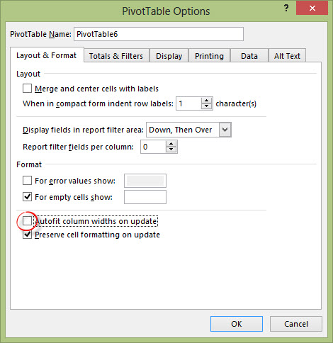
How to make row labels on same line in pivot table? - ExtendOffice Make row labels on same line with PivotTable Options You can also go to the PivotTable Options dialog box to set an option to finish this operation. 1. Click any one cell in the pivot table, and right click to choose PivotTable Options, see screenshot: 2.

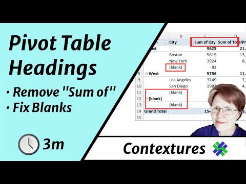
Change Pivot Table Sum of Headings and Blank Labels - YouTube

Design the layout and format of a PivotTable To change the format of the PivotTable, you can apply a predefined style, banded rows, and conditional formatting. Windows Web Mac Changing the layout form of a PivotTable Change a PivotTable to compact, outline, or tabular form Change the way item labels are displayed in a layout form Change the field arrangement in a PivotTable

PHP Pivot Grid / Pivot Table Control | Syncfusion

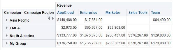
conditional formatting per row on pivot - Microsoft Tech Community conditional formatting per row on pivot. I would like to format each row of a pivot table separately (as in the picture shown below), but I cannot paste the formatting. I've got many rows, and they could change (just like the columns) Is there a way to automate this, or I have to select row by row and apply the formatting?

Finding Duplicates by Using Conditional Formatting in Excel 2010

Pivot Table Grouping, Ungrouping And Conditional Formatting So let's drag the Age under the Rows area to create our Pivot table. #1) Right-click on any number in the pivot table. #2) On the context menu, click Group. #3) Grouping dialog box appears, in this example, the least number is 25, so by default the Starting number is entered as 25, and you can change if necessary.

Lecture - 194 : Excel : Pivot Table part - 6 | Conditional formatting | Right way of number ...

Pivot table conditional formatting based on row label työt Etsi töitä, jotka liittyvät hakusanaan Pivot table conditional formatting based on row label tai palkkaa maailman suurimmalta makkinapaikalta, jossa on yli 21 miljoonaa työtä. Rekisteröityminen ja tarjoaminen on ilmaista.

Finding Duplicates by Using Conditional Formatting in Excel 2010

How to Create a Pivot Table in Power BI - Goodly 19.10.2018 · 2.1 Creating a Tabular / Classic View – Any pivot veteran won’t be able to stand a pivot table without this.If you don’t know, Tabular / Classic View allows each field in rows to occupy a separate column. Here is how a Tabular View looks in a Pivot Table – (I prefer it over classic view) Years and Region – placed in row labels are occupying different columns

Pivot Table Conditional Formatting with VBA - Peltier Tech Blog

Pivot Chart Formatting Changes When Filtered - Peltier Tech 07.04.2014 · If you go to Field Settings for all your row labels in your pivot table and select “show items with no data”, the formatting sticks. The problem is that when you use the slicer, you may have row labels that don’t exist for that intersection, then when you change the slicer, they exist again and Excel puts in the default formatting. If ...

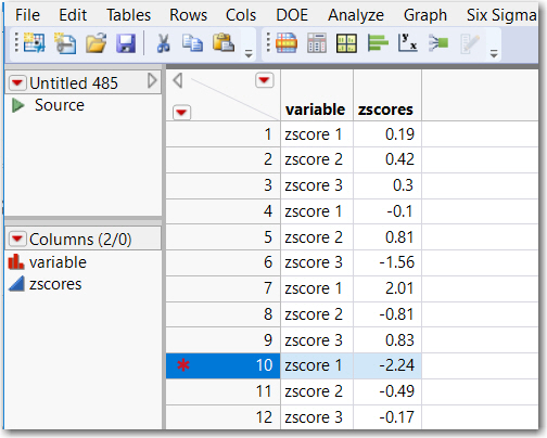
Solved: Conditional Formatting Columns in a Table Box - JMP User Community

Pivot Table Conditional Formatting for Different Rows Items? Bek_from_Uzbekistan. Hello, It is possible! All you have to do: Select Your Pivot Table and: Go to Conditional Formatting -> New Rule -> Choose All cells showing "duration" values for "Type and "Date Selection" under "Apply Rule To" section -> Use a Formula to Determine which cells to format and enter the following formula: =AND (A6="Cars",A6>3),

Finding Duplicates by Using Conditional Formatting in Excel 2010

Conditional Formatting in Pivot Table (Example) | How To Apply? - EDUCBA Click on any cell in the pivot table > Go to the HOME tab > Click on Conditional Formatting option under Styles option > Click on Manage Rules option. It will open a Rules Manager dialog box. Click on the Edit Rule tab, as shown in the below screenshot. It will open the Editing Rule formatting window. Refer to the below screenshot.

Share :