38 excel chart multiple data labels

Per my testing, we may have to manually add it to our data label. The detailed steps are shown in the figure below: But because both Country and Manufacturer columns are category columns, we may not be able to keep only the Country column. Thanks for your understanding. In addition, you can also try to display both in the data bar. How to Add Two Data Labels in Excel Chart (with Easy Steps) You can easily show two parameters in the data label. For instance, you can show the number of units as well as categories in the data label. To do so, Select the data labels. Then right-click your mouse to bring the menu. Format Data Labels side-bar will appear. You will see many options available there. Check Category Name.

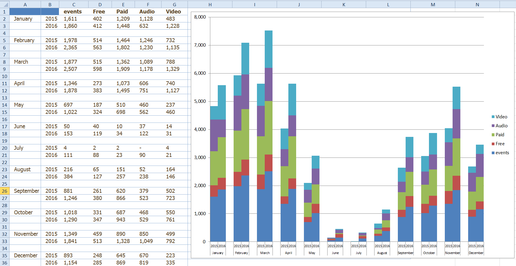
How to Create a Bar Chart in Excel with Multiple Bars? To add data labels, go to the Chart Design ribbon, and from the Add Chart Element, options select Add Data Labels. Adding data labels will add an extra flair to your graph. You can compare the score more easily and come to a conclusion faster. You can also choose a column chart that will give you a similar result.

Excel chart multiple data labels

How to Apply a Filter to a Chart in Microsoft Excel - How-To Geek Select the chart and you'll see buttons display to the right. Click the Chart Filters button (funnel icon). When the filter box opens, select the Values tab at the top. You can then expand and filter by Series, Categories, or both. Simply check the options you want to view on the chart, then click "Apply." How to Create and Customize a Treemap Chart in Microsoft Excel Either right-click the chart and pick "Format Chart Area" or double-click the chart to open the sidebar. On Windows, you'll see two handy buttons on the right of your chart when you select it. With these, you can add, remove, and reposition Chart Elements. And you can pick a style or color scheme with the Chart Styles button. How to Add Total Values to Stacked Bar Chart in Excel The following chart will be created: Step 4: Add Total Values. Next, right click on the yellow line and click Add Data Labels. The following labels will appear: Next, double click on any of the labels. In the new panel that appears, check the button next to Above for the Label Position: Next, double click on the yellow line in the chart.

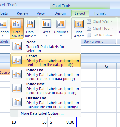
Excel chart multiple data labels. How to Print Labels from Excel - Lifewire Select Mailings > Write & Insert Fields > Update Labels . Once you have the Excel spreadsheet and the Word document set up, you can merge the information and print your labels. Click Finish & Merge in the Finish group on the Mailings tab. Click Edit Individual Documents to preview how your printed labels will appear. Select All > OK . XlDataLabelPosition enumeration (Excel) | Microsoft Docs Microsoft Office Excel 2007 sets the position of the data label. xlLabelPositionCenter-4108: Data label is centered on the data point or is inside a bar or pie chart. xlLabelPositionCustom: 7: Data label is in a custom position. ... Data labels are in multiple positions. › documents › excelHow to add data labels from different column in an Excel chart? This method will guide you to manually add a data label from a cell of different column at a time in an Excel chart. 1.Right click the data series in the chart, and select Add Data Labels > Add Data Labels from the context menu to add data labels. How to Make a Pie Chart in Excel & Add Rich Data Labels to The Chart! 7) With the data point still selected, go to Chart Tools>Format>Shape Styles and click on the drop-down arrow next to Shape Effects and select Shadow and choose Inner Shadow>Inside Diagonal Top Left. 8) With the one data point still selected, right-click this data point, and select Add Data Label>Add Data Callout as shown below.

How to set multiple series labels at once - Microsoft Tech Community Click anywhere in the chart. On the Chart Design tab of the ribbon, in the Data group, click Select Data. Click in the 'Chart data range' box. Select the range containing both the series names and the series values. Click OK. If this doesn't work, press Ctrl+Z to undo the change. 0 Likes Reply Nathan1123130 replied to Hans Vogelaar Excel Dynamic Chart Linked with a Drop-down List Follow the below steps to implement a dynamic chart linked with a drop-down menu in Excel: Step 1: Insert the data set into an Excel sheet in the cells as shown above. Step 2: Now select any cell where you want to create the drop-down list for the courses. Step 3: Now click on the Data tab from the top of the Excel window and then click on Data ... Two-Level Axis Labels (Microsoft Excel) - ExcelTips (ribbon) Excel automatically recognizes that you have two rows being used for the X-axis labels, and formats the chart correctly. Since the X-axis labels appear beneath the chart data, the order of the label rows is reversed—exactly as mentioned at the first of this tip. (See Figure 1.) Figure 1. Two-level axis labels are created automatically by Excel. › plot-multiple-data-sets-onPlot Multiple Data Sets on the Same Chart in Excel Jun 29, 2021 · You can further format the above chart by making it more interactive by changing the “Chart Styles”, adding suitable “Axis Titles”, “Chart Title”, “Data Labels”, changing the “Chart Type” etc. It can be done using the “+” button in the top right corner of the Excel chart.

How to Make a Pie Chart with Multiple Data in Excel (2 Ways) - ExcelDemy First, to add Data Labels, click on the Plus sign as marked in the following picture. After that, check the box of Data Labels. At this stage, you will be able to see that all of your data has labels now. Next, right-click on any of the labels and select Format Data Labels. After that, a new dialogue box named Format Data Labels will pop up. Best Types of Charts in Excel for Data Analysis, Presentation and ... #2 Use a combination chart when you want to compare two or more data series that are not of comparable sizes: #3 Use a combination chart when you want to display different types of data in different ways that can be represented in the same chart. For example, line, bar and column charts can be used on the same chart. 8 Types of Excel Charts and Graphs and When to Use Them - MUO Pie graphs are some of the best Excel chart types to use when you're starting out with categorized data. With that being said, however, pie charts are best used for one single data set that's broken down into categories. If you want to compare multiple data sets, it's best to stick with bar or column charts. 3. DataLabel object (Excel) | Microsoft Docs Use the DataLabel property of the Point object to return the DataLabel object for a single point. The following example turns on the data label for the second point in series one on the chart sheet named Chart1, and sets the data label text to Saturday. On a trendline, the DataLabel property returns the text shown with the trendline.

Excel Charts Archives - PakAccountants.com

Adding Data Labels to Your Chart (Microsoft Excel) - ExcelTips (ribbon) To add data labels in Excel 2013 or later versions, follow these steps: Activate the chart by clicking on it, if necessary. Make sure the Design tab of the ribbon is displayed. (This will appear when the chart is selected.) Click the Add Chart Element drop-down list. Select the Data Labels tool.

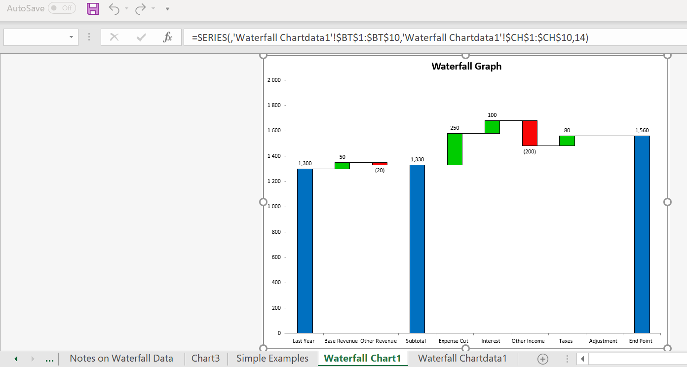
Waterfall Chart Templates (Excel 2010 and 2013) – Edward Bodmer – Project and Corporate Finance

› office-addins-blog › 2015/11/05How to create a chart in Excel from multiple sheets Nov 05, 2015 · If you want to plot data from multiple worksheets in your graph, repeat the process described in step 2 for each data series you want to add. When done, click the OK button on the Select Data Source dialog window. In this example, I've added the 3 rd data series, here's how my Excel chart looks now: 4. Customize and improve the chart (optional)

Enable or Disable Excel Data Labels at the click of a button - How To - PakAccountants.com

Excel: How to Create a Bubble Chart with Labels - Statology Step 3: Add Labels. To add labels to the bubble chart, click anywhere on the chart and then click the green plus "+" sign in the top right corner. Then click the arrow next to Data Labels and then click More Options in the dropdown menu: In the panel that appears on the right side of the screen, check the box next to Value From Cells within ...

excel - How do I update the data label of a chart? - Stack Overflow

Custom Chart Data Labels In Excel With Formulas Follow the steps below to create the custom data labels. Select the chart label you want to change. In the formula-bar hit = (equals), select the cell reference containing your chart label's data. In this case, the first label is in cell E2. Finally, repeat for all your chart laebls.

32 What Is A Data Label In Excel - Labels Design Ideas 2020

Excel Pie Chart Labels on Slices: Add, Show & Modify Factors - ExcelDemy First of all, double-click on the data labels on the pie chart. As a result, a side window called Format Data Labels will appear. Then, go to the drop-down of the Label Options to Label Options tab. After that, check the Percentages option and uncheck all other options. You will get the percentages in the data labels.

How to Add Data Labels on Chart Column in Excel 2007 VID#11 - YouTube

Excel Chart VBA - 33 Examples For Mastering Charts in ... - Analysistabs 30. Set Chart Data Labels and Legends using Excel VBA. You can set Chart Data Labels and Legends by using SetElement property in Excl VBA. Sub Ex_AddDataLabels() Dim cht As Chart 'Add new chart ActiveSheet.Shapes.AddChart.Select With ActiveChart 'Specify source data and orientation.SetSourceData Source:=Sheet1.Range("A1:B5"), PlotBy:=xlColumns ...

How to Create a Chart in Microsoft Excel - TechSupport

peltiertech.com › multiple-time-series-excel-chartMultiple Time Series in an Excel Chart - Peltier Tech Aug 12, 2016 · Start by selecting the monthly data set, and inserting a line chart. Excel has detected the dates and applied a Date Scale, with a spacing of 1 month and base units of 1 month (below left). Select and copy the weekly data set, select the chart, and use Paste Special to add the data to the chart (below right).

Adding data lables to see the value of the bars in an Excel chart

How to Display Percentage in an Excel Graph (3 Methods) Then go to the More Options via the right arrow beside the Data Labels. Select Chart on the Format Data Labels dialog box. Uncheck the Value option. Check the Value From Cells option. Then you have to select cell ranges to extract percentage values. For this purpose, create a column called Percentage using the following formula: =E5/C5

How to Make Excel Charts More Intuitive by Adding Data Labels and Tables - Data Recovery Blog

› 509290 › how-to-use-cell-valuesHow to Use Cell Values for Excel Chart Labels - How-To Geek Mar 12, 2020 · Select the chart, choose the “Chart Elements” option, click the “Data Labels” arrow, and then “More Options.” Uncheck the “Value” box and check the “Value From Cells” box. Select cells C2:C6 to use for the data label range and then click the “OK” button.

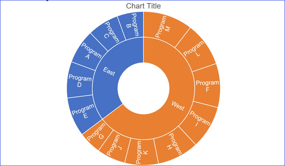
How to Make a Sunburst Chart - ExcelNotes

Chart.ApplyDataLabels method (Excel) | Microsoft Docs Syntax expression. ApplyDataLabels ( Type, LegendKey, AutoText, HasLeaderLines, ShowSeriesName, ShowCategoryName, ShowValue, ShowPercentage, ShowBubbleSize, Separator) expression A variable that represents a Chart object. Parameters Example This example applies category labels to series one on Chart1. VB Copy Charts ("Chart1").SeriesCollection (1).

How to Create a Pie Chart in Microsoft Excel

How to add data labels in excel to graph or chart (Step-by-Step) 1. Select a data series or a graph. After picking the series, click the data point you want to label. 2. Click Add Chart Element Chart Elements button > Data Labels in the upper right corner, close to the chart. 3. Click the arrow and select an option to modify the location. 4.

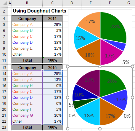
Using Pie Charts and Doughnut Charts in Excel

How To Show Two Sets of Data on One Graph in Excel Choose "All Charts" and click "Combo" as the chart type From the options in the "Recommended Charts" section, select "All Charts" and when the new dialog box appears, choose "Combo" as the chart type. These let Excel know you want to work with multiple data sets before you even edit the graph.

E-xcel Tuts: Add Data Labels to Excel Charts

› comparison-chart-in-excelComparison Chart in Excel | Adding Multiple Series Under Same ... This window helps you modify the chart as it allows you to add the series (Y-Values) as well as Category labels (X-Axis) to configure the chart as per your need. Under Legend Entries ( S eries) inside the Select Data Source window, you need to select the sales values for the year 2018 and year 2019.

Column Chart in Excel - Easy Excel Tutorial

Excel bar chart with multiple series - LeighOrlagh To add data labels go to the Chart Design ribbon and from the Add Chart. Microsoft Excel 2010 Stacked Bar chart with multiple series. Add the weekly values below the monthly values and one column to the right C6C18 with the weekly header in C1. ... Excel Bar Chart With Multiple Series You could make a Multiplication Graph Pub by marking the ...

Excel Dashboard Templates Friday Challenge Answers: Year over Year Chart Comparisons - Excel ...

chandoo.org › wp › change-data-labels-in-chartsHow to Change Excel Chart Data Labels to Custom Values? May 05, 2010 · Now, click on any data label. This will select “all” data labels. Now click once again. At this point excel will select only one data label. Go to Formula bar, press = and point to the cell where the data label for that chart data point is defined. Repeat the process for all other data labels, one after another. See the screencast.

How to Create Multi-Category Chart in Excel - Excel Board

Series.DataLabels method (Excel) | Microsoft Docs Data labels can be turned on or off for individual points in the series. If the series is on an area chart and has the Show Label option turned on for the data labels, the returned collection contains only a single label, which is the label for the area series. Example. This example sets the data labels for series one on Chart1 to show their ...

Sunburst Chart in Excel

How to format axis labels individually in Excel - SpreadsheetWeb Double-click on the axis you want to format. Double-clicking opens the right panel where you can format your axis. Open the Axis Options section if it isn't active. You can find the number formatting selection under Number section. Select Custom item in the Category list. Type your code into the Format Code box and click Add button.

34 Data Label In Excel Chart - Labels For Your Ideas

How to Add Total Values to Stacked Bar Chart in Excel The following chart will be created: Step 4: Add Total Values. Next, right click on the yellow line and click Add Data Labels. The following labels will appear: Next, double click on any of the labels. In the new panel that appears, check the button next to Above for the Label Position: Next, double click on the yellow line in the chart.

Share :